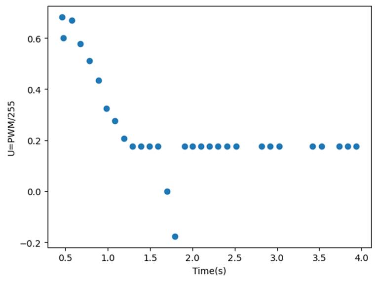
1. Estimate drag and momentum

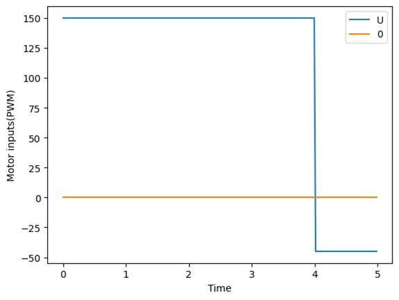
· In this section, I drive the car with a constant PWM for a long enough time to find its steady speed. As the lab7 instruction specified, I originally used active breaking of the car to avoid crashing into the wall: I set the PWM to 150 in the first part of car’s travel, and reuse the functionality from lab 5 to let the car stop in front of the wall to prevent it from breaking in the second part. I modified the code to achieve this combination:

if (curtime < startT + constpwmduration)

{

u = 150;

}

else

{

u = (p + i + d);

                    // deadband

if (0 < u && u < deadband)

{

u = deadband;

}

else if (-deadband < u && u < 0)

{

u = -deadband;

}

else if (u > 255) // motor's range

{

u = 255;

}

else if (u < -255)

{

u = -255;

}

}

setVelocity(u, u);

appendLog(curtime - startT, -1, -1, curpos, -1, p, currealpos, d, dt, u);

where appendLog is function used to store the necessary values in Artemis, its parameters are

appendLog(int timeval, float LPFrollval, float LPFpitchval, float tfsval, float tfs2val, float Pval, float compudistval, float Dval, float dtval, int uval)

-1 is used to fill up the position of parameters that we don’t need in this lab.

· I put the original u=p+i+d part into the else section in the if condition, where the constpwmduration is the duration of the constant PWM value in millisecond; when the condition is true, motor’s PWM is constant 150, when the time pass the set value, the if condition switch PWM to the stop in X meters from wall mode implemented in lab5.

· The way to set constpwmduration is in the jupyter notebook: The command

ble.send_command(CMD.RUN_TO_WALL_STOP,"1500|5000|45|0.78|135|0|50") #constpwmduration|run time|min nonzero speed|velocityfactor|kp|ki|kd

set the constpwmduration =1500 ms, total running time=5000ms.

· However, then I realized that the Time of Flight sensor’s short distance sensoring mode restricts the reliable readings to be with 1.8m, if I persist to include the stop in X meters from wall mode, I wouldn’t have enough distance to confirm the steady speed, so I excluded it by setting constpwmduration to 4000—this time is long enough to ensured PWM is always in the constant value mode until it hit the wall. A paper box is used instead to protect my car. Although, the code above can be useful to achieve protection purposes if TOF sensor use long distance mode.

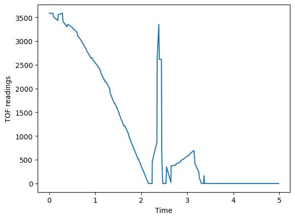
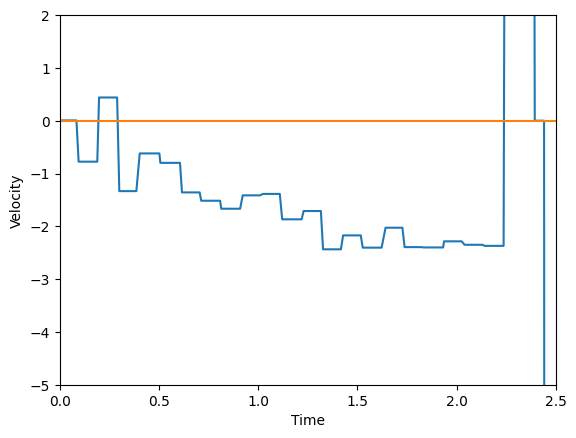
1. The Bluetooth communication codes are the same as lab5. With a same procedure, I got the TOF readings, PWM values, and velocity against the time after driving the car toward the wall with PWM=150:

2. Video of driving to wall:

qqq

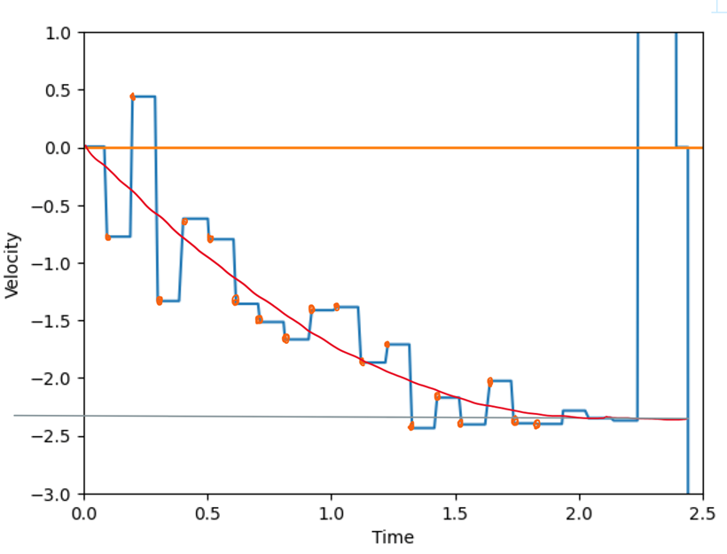
3. Plots:

4. I stored the data collected to Lab7_data.csv using Pandas:

import pandas as pd

df = pd.DataFrame({

'Time': timels,

'TOF': tfls,

'Motor inputs(PWM)': uls,

'Velocity': vells

})

# Save to CSV

df.to_csv('Lab7_data.csv', index=False)

5. and extract them back when needed:

df = pd.read_csv('Lab7_data.csv')

timels = df['Time'].to_numpy()

tfls = df['TOF'].to_numpy()

uls = df['Motor inputs(PWM)'].to_numpy()

vells = df['Velocity'].to_numpy()

6. According to the data, the car hits the wall at t =2.165, so only the data before t=2.165 are meaningful for me.

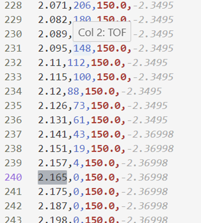
The csv data shown above are Time, TOF, PWM, velocity respectively.

7. By looking at the plots and averaging the last 3 unique meaning Velocity value in csv, I found that the steady speed =(-2.2843-2.3495-2.36998)/3=-2.35632 m/s, Tsteady=2.04 s; Thus 90% rise time = 2.04*0.9=1.836 s, and the speed at 90% risetime = -2.40.

2. Initialize KF (Python)

8. Computing d and m :

o d=u/steady speed =1/ steady speed (since we assume u=1) = 1/2356.32 mm/s

o m=-d*t_0.9/ln(1-0.9)= -1/2356.32*1.836/ln(0.1)= 3.3839405 *10^4

9. Matrix A and B:

o Our state space equation is:

§

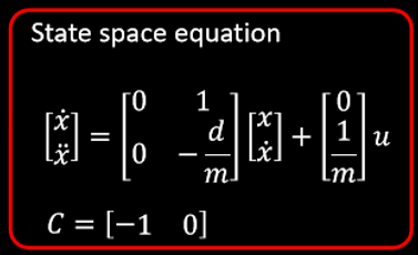
So A= [ [0,1], [0,-d/m] ] = [ [0,1], [0,-d/m] ]= [[ 0, 1, ] [ 0, -1.25413131 ] ], B= [[0], [1/m]] =[ [0], [2955.1346]], C=[-1,0]. They are all stored in array since NumPy provides lots of powerful functions.

10. Process noise and sensor noise

o Determine the delta_t between each TOF sensor readings

§ The car sends back all TOF sensor readings (the ones without interpolation) to python through Bluetooth, but that includes repetitive readings, so I implemented the codes below to remove the repetitive parts and use the list of unique TOF readings to construct an array of time stamps when these TOF readings are recorded; the array of PWM and TOF readings are also constructed along with the time array as they will also be used later; the array of u, tuz[1], is divided by 255 to convert its range to [0,1]:

# realposar: real position array

realposar = np.array(realposls)

# tuzls = the list of time, u(=control=PWM inputs), z(=observation=TOF readings) of each unique TOF sensor readings

# e.g. tuz[0] = a list of time of each unique TOF sensor readings

tuzls = [[], [], []]

prepos = 0

for i, pos in enumerate(realposar):

if prepos != pos:

tuzls[0].append(timels[i])

tuzls[1].append(uls[i])

tuzls[2].append(pos)

prepos = pos

tuz = np.array(tuzls)

tuz[1] /= 255

§ Then call diff() to convert time array to delta_t array.

dtar_tof = np.diff(tuz[0])

o Compute sigma_u and sigma_z

§ The average of my dtar_tof, the array of the dt between each TOF reading, was 0.11986 s; Substitute the average into the model below and got sigma_2=sigma_1= 28.884:

sigma_1=np.sqrt(10**2/np.average(dtar_tof))

sigma_2=sigma_1

sigma_3=20 # all length are in mm, but all time are in s

· The position model used here is from lecture slides:

o

§ Plug sigma1,2,3 into the matrix:

sigma_u=np.array([[sigma_1**2,0],[0,sigma_2**2]])

sigma_z=np.array([[sigma_3**2]])

3. Implement and test your Kalman Filter in Jupyter (Python)

a. Implement the KF() function

o The function is defined below. it has two parts: prediction and updating. Since dt for each step may be different, I updated it by including dt in the parameters. In prediction part, I compute the Ad and Bd from A and B, then use Ad, Bd, previous state (mu & sigma) along with motor inputs and its stddev to predict the prediction state (mu_p & sigma_p); In updating stage, the prediction states is updated with the observation from TOF sensor. The kkf_gain shows how much I trust TOF’s readings: the higher the kkf_gain is, the more I trust TOF readings.

def kf(mu,sigma,u,z, dt):#mu and sigma are the prior state; u is control, z is observation(sensor reading)

#prediction: produce a prediction based on the prior state&control

Ad=np.eye(2) + dt*A

Bd=dt*B

mu_p = Ad.dot(mu) + Bd.dot(u)    

sigma_p = Ad.dot(sigma.dot(Ad.transpose())) + sigma_u

#update: use obvservation to update the prediction

sigma_m = C.dot(sigma_p.dot(C.transpose())) + sigma_z

kkf_gain = sigma_p.dot(C.transpose().dot(np.linalg.inv(sigma_m)))

mu = mu_p + kkf_gain.dot(z-C.dot(mu_p))   # a formula that denoises mu

sigma=(np.eye(2)-kkf_gain.dot(C)).dot(sigma_p)  # a formula that denoises sigma

return mu,sigma, mu_p

b. Choose the initial state of KF readings

o The Kalman Filter need previous state to work, so the initial state must be given before kf() is called, it is defined as follows, where mu_kf starts with TOF’s 1st reading and the initial velocity, and var_kf starts with empirical value ([[20, 20], [20, 20]]

# final len(kf) should==num+1

# kf=[mu list, sigma list]

mu_kf = [np.array([[tuz[2][0]],[vells[0]]]),]

var_kf = [np.array([[20, 20], [20, 20]]),]

c. Loop through all steps and get KF result

o Last, call KF after each step to predict the next one:

_, num = np.shape(tuz)

#num-1 since dt is 1 less than length of time,u,z

mu_p_ls=[np.array([[tuz[2][0]],[vells[0]]]),]

for i in range(num-1):

mu, sigma,mu_p = kf(mu_kf[i], var_kf[i], tuz[1][i], -tuz[2][i],dtar_tof[i])

mu_kf.append(mu)

var_kf.append(sigma)

mu_p_ls.append(mu_p)

o Plot the result:

§

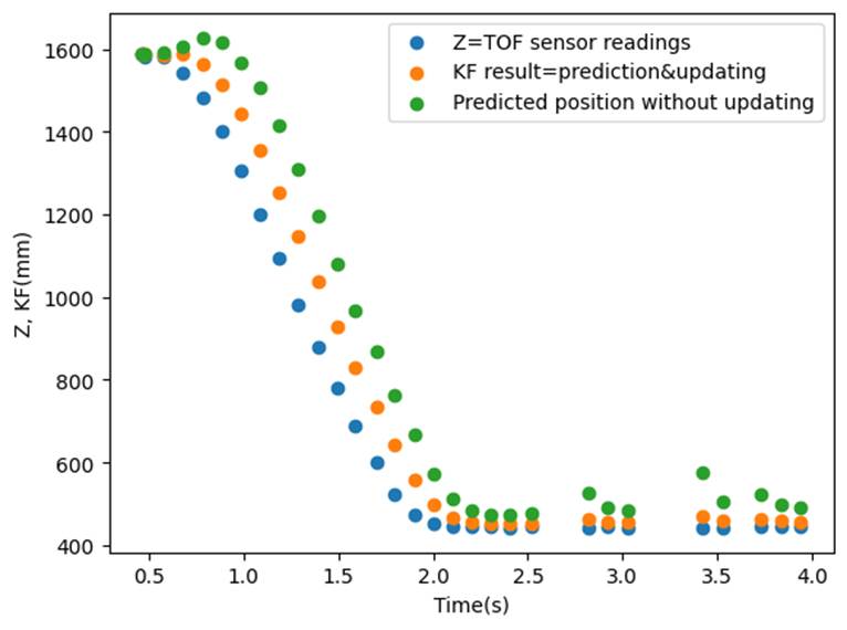
§ As the plot show, the prediction is made and then updated successfully; the KF result is very close to the TOF readings,

§ The U’s plot is consistent with the curves above:

§